← Projects Research · UT Dallas · 2025

Predicting Ocean Wave Forces with CNNs

Joint first author · Flow Dynamics and Turbulence Lab, UT Dallas

Convolutional neural networks that predict the force of ocean waves hitting an offshore monopile. We built the training data from 64 large-eddy simulations run through an automated supercomputer pipeline. Each simulation takes hours of supercomputer time; the trained network answers in under a second.

Published · ASME OMAE 2026 CNN-Based Prediction of Ocean Wave Impact Forces on Monopile Structures Max Liu^†, Vedant Mohapatra^†, Ahmed A. Hamada, Rituja Kulkarni, Stefano Leonardi, Kianoosh Yousefi († joint first authors) Proceedings of the ASME 2026 International Ocean, Offshore and Arctic Engineering Conference (OMAE2026), June 7–12, 2026, Tokyo, Japan · Paper OMAE2026-176039

Read on ASME Digital Collection → DOI: 10.1115/OMAE2026-176039 Code on GitHub → View poster ↓

Simulated wave impacting a vertical cylinder, colored by velocity magnitude, with the clustered mesh visible — Large-eddy simulation of a wave hitting the monopile, colored by velocity magnitude, with the refined mesh around the cylinder

64LES simulations

3CNNs: force values, force profile, pressure map

12.4%mean error, paper model

<1 sper prediction

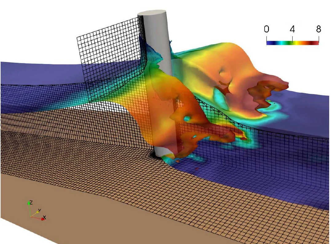
Why it matters

Offshore wind turbines, oil platforms and bridge piers take repeated wave impacts that drive structural fatigue over decades.
High-fidelity simulations capture these forces accurately but are far too slow for design studies or real-time monitoring.
Goal: learn the mapping from an incoming wave to the force it produces, so the force can be predicted almost instantly.

What the models learn $$\mathcal{M} : \eta(t) \;\rightarrow\; F(t),\; p(z, \theta)$$

$\eta(t)$: free-surface elevation of the incoming wave over 40 s
$F(t)$: inline force on the monopile over one wave period
$p(z,\theta)$: mean pressure on the cylinder surface by height and angle

Summer 2025 · STEM Bridge ProgramJun–Aug
- Four students picked 64 wave cases, ran 16 simulations each on the Ganymede2 cluster, wrote the post-processing code and trained three CNNs. The work was presented as a poster.
Paper · ASME OMAE 2026Published
- Stricter simulation settings, validation against published data and a regularized force-profile CNN, published with Max Liu as joint first author.

01 · Choosing the wave cases

Which wave theory applies depends on how deep the water is relative to the wavelength and how steep the wave is. A MATLAB script draws the standard wave-theory diagram in those two dimensionless numbers (Airy, Stokes II–V, cnoidal, solitary and breaking regions, with the Ursell-number boundary) and places candidate cases on it.

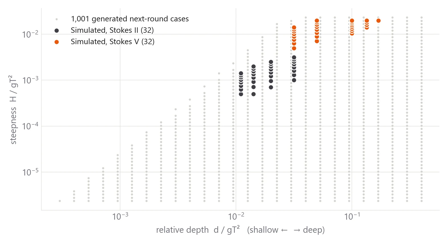
Log-log plot of wave steepness against relative depth: 32 Stokes II and 32 Stokes V simulated cases in the middle, and a grid of about 1,000 generated cases spread across the region — The 64 simulated cases, and the 1,001-case grid generated for the next round, on the wave-theory diagram (water depth d = 3.8 m)

64 cases: 8 wave periods from 1.51 to 5.94 s, each with 8 heights from 0.12 to 1.70 m.
Stokes II for the 32 gentler waves and Stokes V for the 32 steeper ones.
Next round: the script fills the region between the Ursell-number limit and the Stokes V limit with a log-spaced 26 × 58 grid. It keeps the 1,001 points inside the region and writes their periods and heights to a CSV.
Python then generated a case folder for each of those 1,001 points on a medium mesh (1.5× the base resolution in each direction, with a 2× fine version also set up). They are ready for a larger dataset but haven't been run.

Diagram axes and Ursell number $$\frac{d}{gT^2}, \qquad \frac{H}{gT^2}, \qquad U_r = \frac{H L^2}{d^3}$$

$d, H, T, L$: water depth, wave height, period and wavelength
$U_r = 26$: boundary between Stokes-type and cnoidal (shallow) waves

02 · Simulations

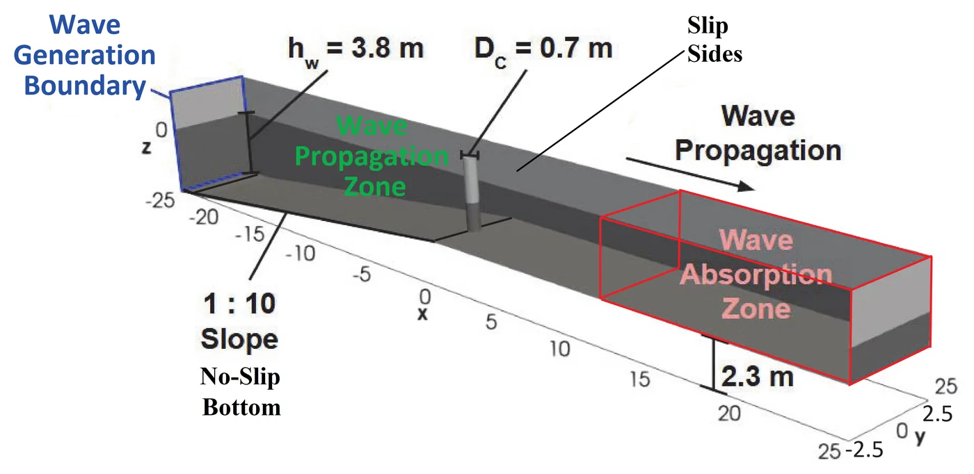
Schematic of the 50 m numerical wave tank with a 1:10 slope and a vertical cylinder — Numerical wave tank: waves generated at the inlet run up a 1:10 slope and hit a 0.7 m cylinder

Solver: OpenFOAM interFoam: large-eddy simulation with volume-of-fluid for the air–water interface
Domain: 50 m tank, 3.8 m still-water depth at the wavemaker, 1:10 sloped seabed, 0.7 m cylinder where the depth is 1.5 m
Waves: Stokes II or V generated at the inlet with a 1 s ramp and active absorption; absorbing outlet to stop reflections
Fluids: Water at 20 °C (998.19 kg/m³) and air, with surface tension
Mesh: Block mesh refined three times around the free surface and cylinder; the paper's mesh has about 1.46 million cells, down to 5 mm
Run: 40 s of simulated time per case with an adaptive time step capped by a Courant number limit
Recorded: Force on the cylinder every time step, water height at five wave gauges, time-averaged velocity and pressure, and the mean surface pressure every 5 s
Compute: 128 cores and 256 GB per case on Ganymede2 (UT Dallas); about a month of cumulative wall-clock time for all 64

Normalized force time history compared with Li and Fuhrman reference data — Validation: computed force on the cylinder vs. published reference data (Li & Fuhrman)

03 · Automated pipeline

Setting up, submitting and collecting 64 cases by hand would have been slow and error-prone, so each step was scripted. Each student copied a template case 16 times, and the scripts did the rest.

Set up
1
Domain and mesh creationOpenFOAM

blockMesh builds the tank, three passes of topoSet + refineMesh refine around the waves and cylinder, and setFields fills in the water.
2
Make 64 unique wave casesMATLAB

Height, period and Stokes order for each case, picked on the wave-theory diagram and split 16 per student.
3
Regex code to auto-update every casePython

Rewrites each copy's wave height, period and Stokes order and renames its SLURM job, so no file is edited by hand.
Run on Ganymede2
4
Make SLURM script and submit jobSLURM

decomposePar splits the mesh into 128 pieces (4 × 4 × 8), and each case runs interFoam on one 128-core node in the preemptible queue (2-day limit).
5
Reconstruct the case once completeOpenFOAM

reconstructPar merges the 128 processor pieces back into one case.
6
Combine data from paused jobs29 of 64 restarted

Preempted jobs resume from the latest saved time, and each restart writes a new output folder. The pieces are joined back into one 40 s record.
Collect
7
Extract raw force dataPython

Copies each case's force, wave-gauge and surface-pressure output into one folder per case for post-processing.

04 · Post-processing

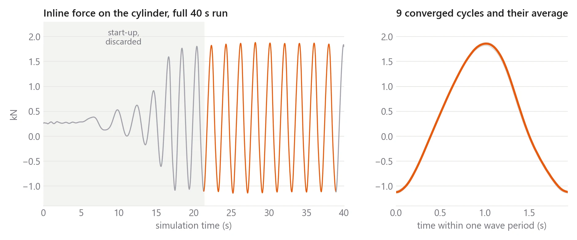
Python scripts turn each run's raw output into training targets. The early part of every run is a start-up transient, so only fully developed, converged wave cycles are kept.

Left: inline force over a 40 s run, growing during start-up then settling into regular cycles that are kept. Right: nine kept cycles overlaid with their average — One of the 64 cases (H = 0.61 m, T = 1.97 s, Stokes V): the start-up is dropped, and the converged cycles average into one force profile

Parse: read the force file into total, pressure and viscous inline force, rejoining the segments of restarted runs.
Find cycles: a sliding window marks local peaks and troughs. The start-up is dropped once successive troughs settle to a steady value, and incomplete cycles at the end are trimmed.
Force values: mean, max and min of the total, pressure and viscous force, giving 9 numbers per case.
Force profile: an FFT finds the dominant period, every kept cycle is folded onto one period, averaged into 3,000 points and lightly smoothed.
Pressure map: the mean pressure sampled on the cylinder surface is converted from x, y to angle and gridded into 328 heights × 160 angles.
Inputs: each case's wave elevation is computed from its Stokes theory over the 40 s run and sampled at 3,000 points.

Phase average and normalization $$\bar{F}(\phi) = \frac{1}{N}\sum_{k=1}^{N} F\!\left(t_k + \phi\,T\right), \qquad \hat{x} = 2\,\frac{x - x_{\min}}{x_{\max} - x_{\min}} - 1$$

$t_k, N$: start of each kept cycle, number of cycles
$\phi$: phase within the wave period $T$, from 0 to 1
$\hat{x}$: every input and output scaled to [−1, 1] before training

05 · Three CNNs

All three take the same input: the 3,000-point wave elevation. They differ in what they predict, so each has its own output head. They were built in TensorFlow/Keras with a fixed random seed. 10% of cases were held out as a blind test set, and 10% of the rest were used for validation.

Model	Predicts	Network	Parameters
Force values	Mean, max and min of total, pressure and viscous force (9 outputs)	3 conv blocks (8, 16, 32 filters, stride 3) with batch norm and max pooling, then dense 64	17,257
Force profile	Force over one wave period (3,000 outputs)	Same backbone with a 3,000-unit output layer	211,672
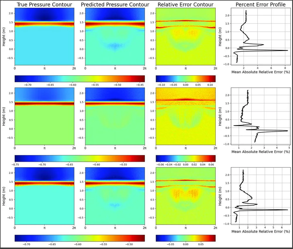
Pressure map	Mean pressure on the cylinder (328 × 160 grid)	4 conv blocks (16, 32, 64, 128 filters), dense 64, then a 52,480-unit layer reshaped to the grid	5,056,576

Adam optimizer, mean-squared-error loss, up to 200 epochs, learning rate cut by 10% after 10 epochs without improvement; the pressure model also stops early.
Training error on the normalized data averaged an MAE of 0.013. Validation error was higher (MAE 0.11 for force values, 0.17 for the profile, 0.027 for pressure), so with 64 cases the models overfit, which is what the paper version targets.

True vs predicted mean pressure contours on the cylinder with relative error — Pressure-map CNN on held-out cases: true vs. predicted mean pressure around the cylinder, with the error

06 · Refining for the paper

The paper focuses on the force profile and tightens both the simulations and the network.

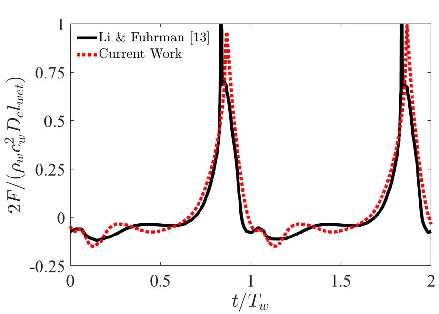
Simulations: the maximum Courant number dropped from 0.65 to 0.05, the subgrid model is WALE, and the force history was validated against Li & Fuhrman.
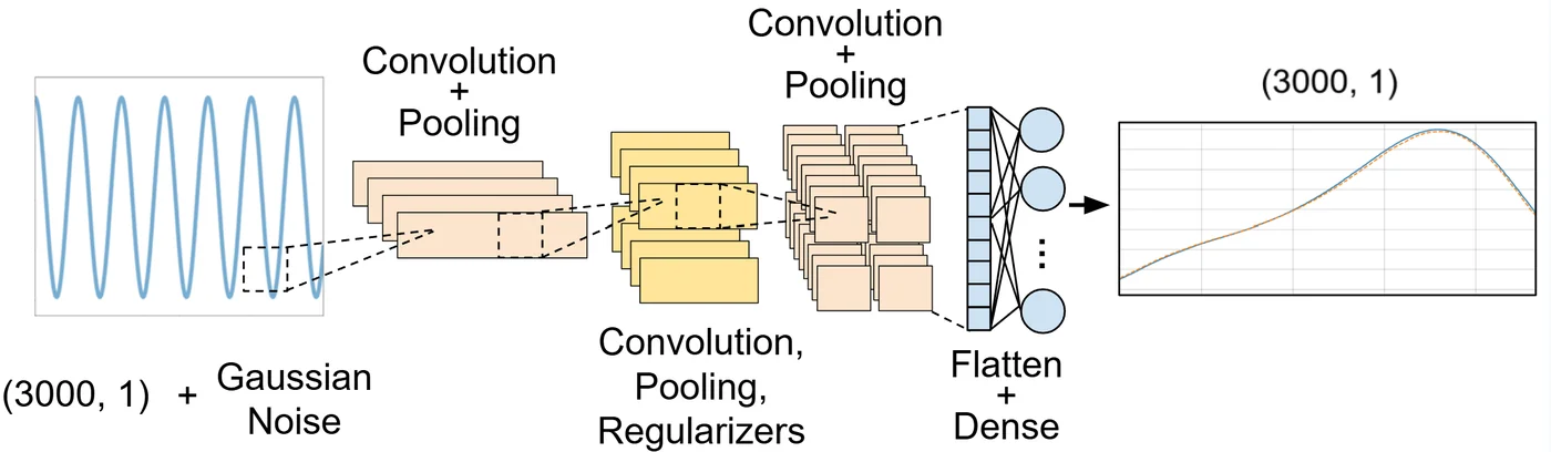
Network: Gaussian input noise, three convolution + average-pooling blocks (16, 32, 64 filters), dense layers of 32, 64 and 128, and a 3,000-point output.
Training: L1/L2 regularization, Adam and k-fold cross-validation, with an 80 / 10 / 10 split for training, validation and blind testing.

CNN architecture: 3000-point wave input with Gaussian noise, convolution and pooling blocks, dense layers, 3000-point force output — Paper model: 3,000-point wave signal in, 3,000-point force profile out

07 · Results

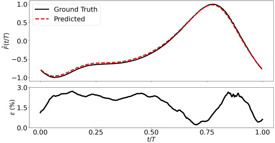
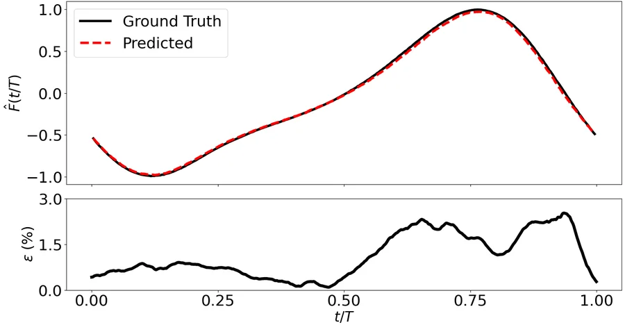
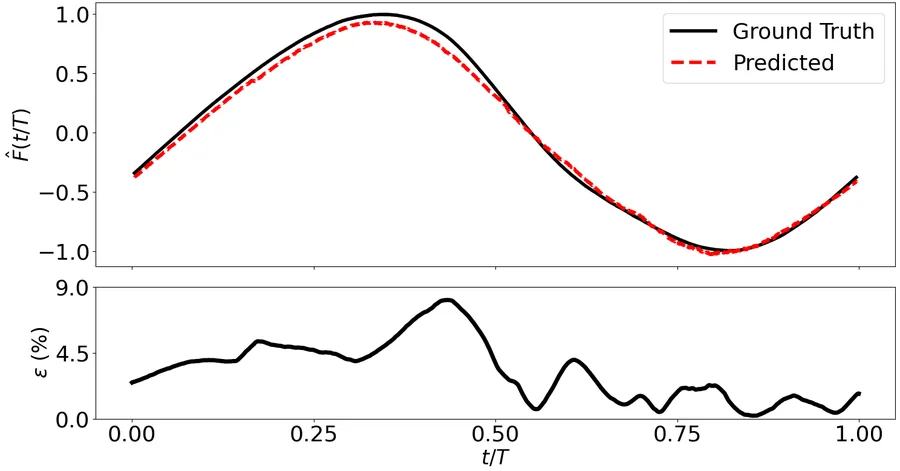
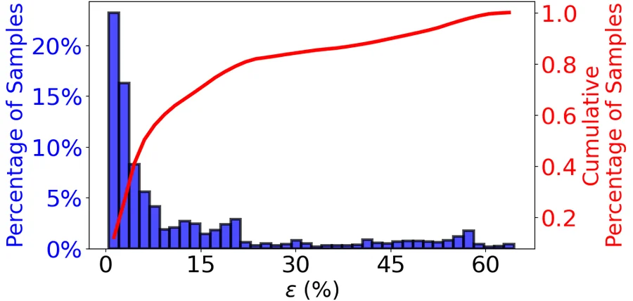
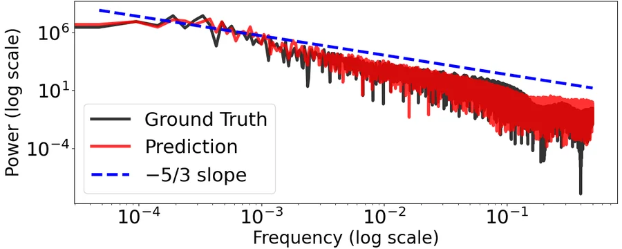
On blind test cases the paper's CNN reproduces the impact peak, run-up and decay of the force with a mean error of 12.4%. About 80% of unseen samples fall within 20% error.

Test case 1

Test case 2

Test case 3

Histogram of prediction error across test samples — Error distribution, concentrated near zero

Power spectral density of predicted and true force — Spectra match where the force energy is (f < 0.15)

Cross-correlation between predicted and true force — 0.82 correlation peak at zero lag

Error metric (normalized arctangent) $$\epsilon = \frac{\tan^{-1}\left|\hat{F}^{GT}_i - \hat{F}^{P}_i\right|}{\pi/2}$$

Poster

Presented through the UT Dallas STEM Bridge Program with Max Liu, Annie Yang and Amy Yang, covering all three summer CNNs.

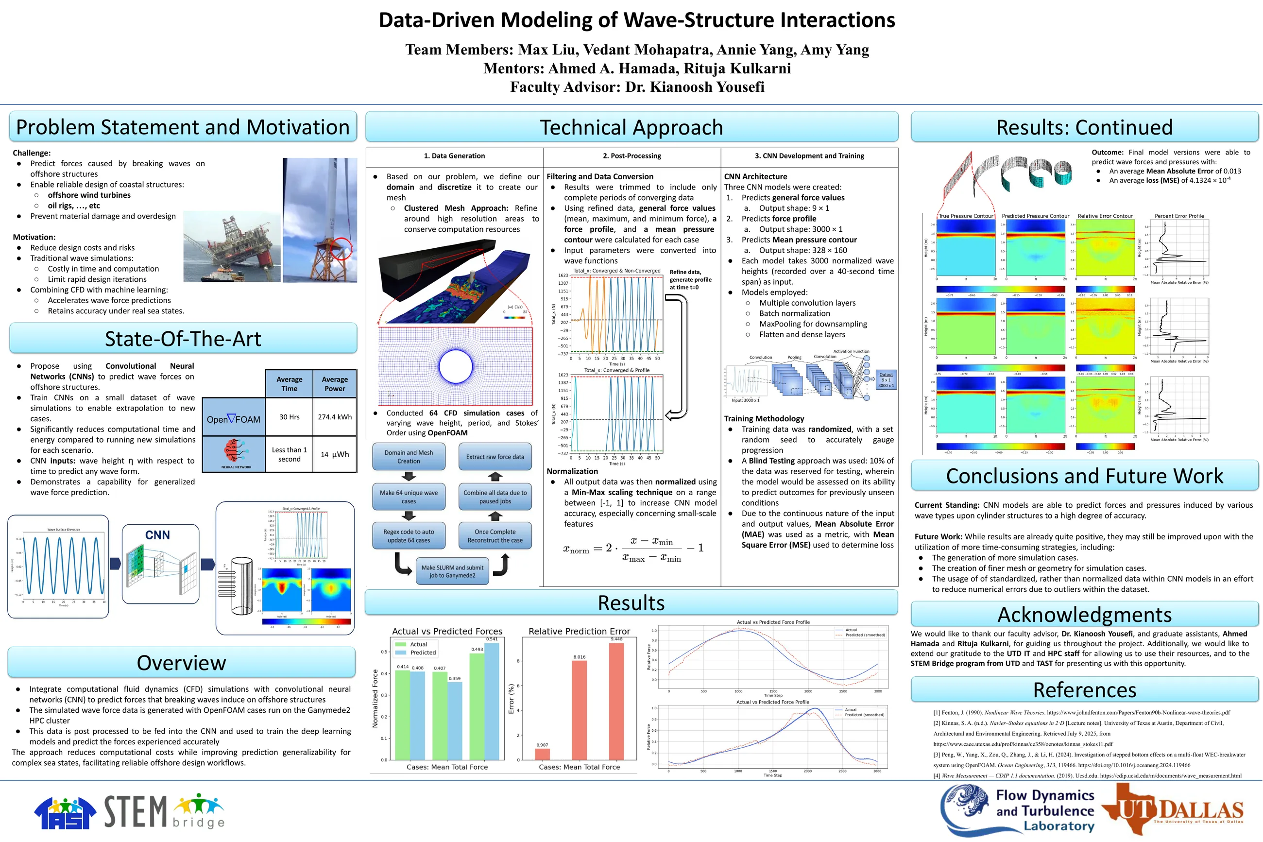
Method	Time	Energy
CFD simulation (OpenFOAM)	About 30 hours on a cluster	274.4 kWh
CNN prediction	< 1 second	14 μWh

Acknowledgments

Advised by Dr. Kianoosh Yousefi with mentors Ahmed A. Hamada and Rituja Kulkarni. Supported by the National Science Foundation (grant 2404368), with computing from HPC@UTD and student participation through the UT Dallas STEM Bridge Program and TAST.